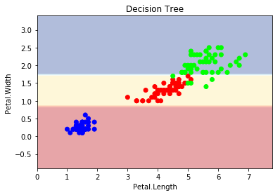
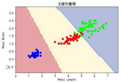
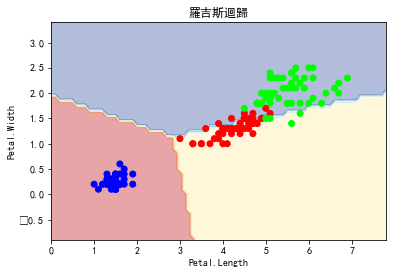
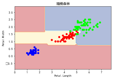
import matplotlib.pyplot as plt from sklearn.datasets import load_iris from sklearn import tree from sklearn.svm import SVC from sklearn.linear_model import LogisticRegression from sklearn.ensemble import RandomForestClassifier matplotlib.rc('font', **{'sans-serif' : 'SimHei', 'family' : 'sans-serif'}) def plot_estimator(estimator, X, y, title): x_min, x_max = X[:, 0].min() - 1, X[:, 0].max() + 1 y_min, y_max = X[:, 1].min() - 1, X[:, 1].max() + 1 xx, yy = np.meshgrid(np.arange(x_min, x_max, 0.1), np.arange(y_min, y_max, 0.1)) Z = estimator.predict(np.c_[xx.ravel(), yy.ravel()]) Z = Z.reshape(xx.shape) plt.plot() plt.contourf(xx, yy, Z, alpha=0.4, cmap = plt.cm.RdYlBu) plt.scatter(X[:, 0], X[:, 1], c=y, cmap = plt.cm.brg) plt.title(title) plt.xlabel('Petal.Length') plt.ylabel('Petal.Width') plt.show() iris = load_iris() X = iris.data[:,[2,3]] y = iris.target[:] clf = tree.DecisionTreeClassifier() clf.fit(X, y) clf1 = SVC(kernel="linear") clf1.fit(X, y) clf2 = LogisticRegression() clf2.fit(X, y) clf3 = RandomForestClassifier(n_estimators=100, criterion="entropy", random_state=0) clf3.fit(X, y) plot_estimator(clf, X, y, "決策樹") plot_estimator(clf1, X, y, "支援向量機") plot_estimator(clf2, X, y, "羅吉斯迴歸") plot_estimator(clf3, X, y, "隨機森林")
|