相關係數,線性迴歸, statsmodels, sklearn, itertools
相關係數 rets.corr()
Ctrip
Lion
Ctrip
1.000000
0.059657
Lion
0.059657
1.000000
1
2
3
4
5
6
7
8
9
10
11
12
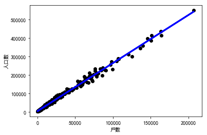
from sklearn.linear_model import LinearRegression
X1 = X.iloc[0 :len(X)].to_frame()
Y1 = Y.iloc[0 :len(Y)].to_frame()
regr = LinearRegression()
regr.fit(X1,Y1)
regr.coef_
regr.intercept_
regr.predict(X1)
% pylab inline
plt.scatter(X1,Y1, color="black" )
plt.xlabel('戶數' ,fontproperties='SimHei' )
plt.ylabel('人口數' ,fontproperties='SimHei' )
$$ Y = \beta_0+\beta_1X $$
錯誤訊息:Found input variables with inconsistent numbers of samples: [1, 368]
series 是一維的數據類型,dataframe 是一個二維的、表格型的數據結構。
多變量線性迴歸 `線性迴歸也被稱為最小二乘法回歸(Linear Regression, also called Ordinary Least-Squares (OLS) Regression)
sklearn 1
2
3
4
5
6
7
8
9
10
house = pd.read_csv('python_for_data_science-master/Data/house-prices.csv' )
house1 = pd.concat([house,pd.get_dummies(house['Brick' ]),pd.get_dummies(house['Neighborhood' ])],axis=1 )
del house1['Home' ], house1['No' ], house1['Brick' ], house1['Neighborhood' ]
X = house1[['SqFt' , 'Bedrooms' , 'Bathrooms' , 'Offers' , 'Yes' , 'East' , 'North' , 'West' ]]
Y = house1['Price' ].values
from sklearn.linear_model import LinearRegression
regr = LinearRegression()
regr.fit(X,Y)
house1['Price_Predict' ] = regr.predict(X).astype(int)
house1.head()
Price
SqFt
Bedrooms
Bathrooms
Offers
Yes
East
North
West
Price_Predict
0
114300
1790
2
2
2
0
1
0
0
103182
1
114200
2030
4
2
3
0
1
0
0
116127
2
114800
1740
3
2
1
0
1
0
0
113047
3
94700
1980
3
2
3
0
1
0
0
109230
4
119800
2130
3
3
3
0
1
0
0
125063
statsmodels 參數估計:
1
2
3
4
5
import statsmodels.api as sm
X2 = sm.add_constant(X)
est = sm.OLS(Y, X2)
est2 = est.fit()
print (est2.summary())
sklearn,statsmodels計算之結果是相同的
regr.coef_
regr.intercept_
est2.params
赤池信息準則 AIC (Akaike Information Criterion) 評估統計模型的複雜度和衡量統計模型「擬合」資料之優良性的一種標準,尋找可以最好地解釋數據但包含最少自由參數的模型,優先考慮的模型應是AIC值最小的那一個
貝葉斯信息準則 SIC (Schwartz Information Criterion)
1
2
3
4
5
6
7
8
9
10
11
12
13
predictorcols = ['SqFt', 'Bedrooms', 'Bathrooms', 'Offers', 'Yes', 'East', 'North']
import itertools
AICs = {}
for k in range(1,len(predictorcols)+1):
for variables in itertools.combinations(predictorcols, k):
predictors = X[list(variables)]
predictors2 = sm.add_constant(predictors)
est = sm.OLS(Y, predictors2)
res = est.fit()
AICs[variables] = res.aic
from collections import Counter
c = Counter(AICs)
c.most_common()[::-10] #x[startAt:endBefore:skip]
itertools迭代指重覆取值,重覆反饋過程的活動itertools.combinations(['A','B','C','D'],2)可以得到AB,AC,AD,BC,BD,CD
1
2
3
4
5
6
7
8
============== ==== ==== ======= ===== ====================
Min Max Mean SD Class Correlation
============== ==== ==== ======= ===== ====================
sepal length: 4.3 7.9 5.84 0.83 0.7826
sepal width: 2.0 4.4 3.05 0.43 -0.4194
petal length: 1.0 6.9 3.76 1.76 0.9490 (high!)
petal width: 0.1 2.5 1.20 0.76 0.9565 (high!)
============== ==== ==== ======= ===== ====================
上述為iris資料庫之描述性統計資料,下面取petal length及petal width使用,分別取最小值及最大值後加減1,並進行meshgrid處理
1
2
3
4
5
6
7
8
9
10
11
12
13
14
15
16
17
18
19
20
21
22
23
24
25
26
27
28
29
30
31
32
33
34
35
36
37
38
39
40
41
42
43
44
45
46
47
48
49
import matplotlib.pyplot as plt
from sklearn.datasets import load_iris
from sklearn import tree
from sklearn.svm import SVC
from sklearn.linear_model import LogisticRegression
from sklearn.ensemble import RandomForestClassifier
matplotlib.rc('font' , **{'sans-serif' : 'SimHei' ,
'family' : 'sans-serif' })
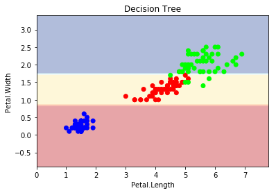
def plot_estimator (estimator, X, y, title) :
x_min, x_max = X[:, 0 ].min() - 1 , X[:, 0 ].max() + 1
y_min, y_max = X[:, 1 ].min() - 1 , X[:, 1 ].max() + 1
xx, yy = np.meshgrid(np.arange(x_min, x_max, 0.1 ),
np.arange(y_min, y_max, 0.1 ))
Z = estimator.predict(np.c_[xx.ravel(), yy.ravel()])
Z = Z.reshape(xx.shape)
plt.plot()
plt.contourf(xx, yy, Z, alpha=0.4 , cmap = plt.cm.RdYlBu)
plt.scatter(X[:, 0 ], X[:, 1 ], c=y, cmap = plt.cm.brg)
plt.title(title)
plt.xlabel('Petal.Length' )
plt.ylabel('Petal.Width' )
plt.show()
iris = load_iris()
X = iris.data[:,[2 ,3 ]]
y = iris.target[:]
clf = tree.DecisionTreeClassifier()
clf.fit(X, y)
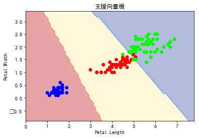
clf1 = SVC(kernel="linear" )
clf1.fit(X, y)
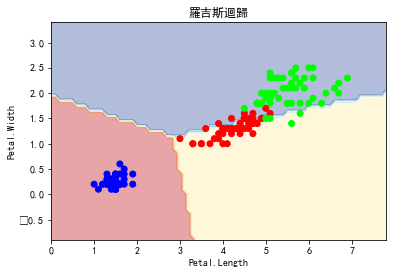
clf2 = LogisticRegression()
clf2.fit(X, y)
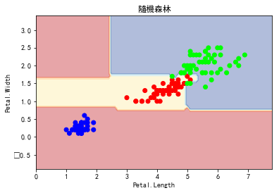
clf3 = RandomForestClassifier(n_estimators=100 , criterion="entropy" , random_state=0 )
clf3.fit(X, y)
plot_estimator(clf, X, y, "決策樹" )
plot_estimator(clf1, X, y, "支援向量機" )
plot_estimator(clf2, X, y, "羅吉斯迴歸" )
plot_estimator(clf3, X, y, "隨機森林" )
The C parameter tells the SVM optimization how much you want to avoid misclassifying each training example. For large values of C, the optimization will choose a smaller-margin hyperplane if that hyperplane does a better job of getting all the training points classified correctly. Conversely, a very small value of C will cause the optimizer to look for a larger-margin separating hyperplane, even if that hyperplane misclassifies more points. For very tiny values of C, you should get misclassified examples, often even if your training data is linearly separable.
傳統線性迴歸的迴歸係數(regression coefficient)的解釋為「當自變項增加一個單位,依變項則會增加多少單位」,但是在Logistic regression的迴歸係數解釋為「當自變項增加一個單位,依變項1相對依變項0的機率會增加幾倍」,也就是說「自變項增加一個單位,依變項有發生狀況(習慣稱為Event)相對於沒有發生狀況(non-event)的比值」,這個比值就是勝算比(Odds ratio, OR)。我們可以這樣說,除了迴歸係數的解釋方法不太相同之外,基本上可說傳統線性迴歸跟Logistic regression是一樣的分析。晨晰統計
顧客忠誠度分析 1
2
3
4
5
6
state account_length area_code international_plan voice_mail_plan number_vmail_messages total_day_minutes total_day_calls total_day_charge total_eve_minutes total_eve_calls total_eve_charge total_night_minutes total_night_calls total_night_charge total_intl_minutes total_intl_calls total_intl_charge number_customer_service_calls churn
1 KS 128 area_code_415 no yes 25 265.1 110 45.07 197.4 99 16.78 244.7 91 11.01 10.0 3 2.70 1 no
2 OH 107 area_code_415 no yes 26 161.6 123 27.47 195.5 103 16.62 254.4 103 11.45 13.7 3 3.70 1 no
3 NJ 137 area_code_415 no no 0 243.4 114 41.38 121.2 110 10.30 162.6 104 7.32 12.2 5 3.29 0 no
4 OH 84 area_code_408 yes no 0 299.4 71 50.90 61.9 88 5.26 196.9 89 8.86 6.6 7 1.78 2 no
5 OK 75 area_code_415 yes no 0 166.7 113 28.34 148.3 122 12.61 186.9 121 8.41 10.1 3 2.73 3 no
電信公司之客戶忠誠度分析資料
1
2
3
4
5
6
7
8
9
10
11
12
13
14
15
16
17
18
19
20
21
22
23
24
25
26
27
28
import pandas
import numpy
from sklearn import tree
from sklearn.tree import export_graphviz
import graphviz
import pydotplus
df = pandas.read_csv('python_for_data_science-master/Data/customer_churn.csv' , index_col=0 , header = 0 )
df = df.iloc[:,3 :]
cat_var = ['international_plan' ,'voice_mail_plan' , 'churn' ]
for cat in cat_var:
df[cat] = df[cat].map(lambda e: 1 if e == 'yes' else 0 )
y = df.iloc[:,-1 ]
X = df.iloc[:,:-1 ]
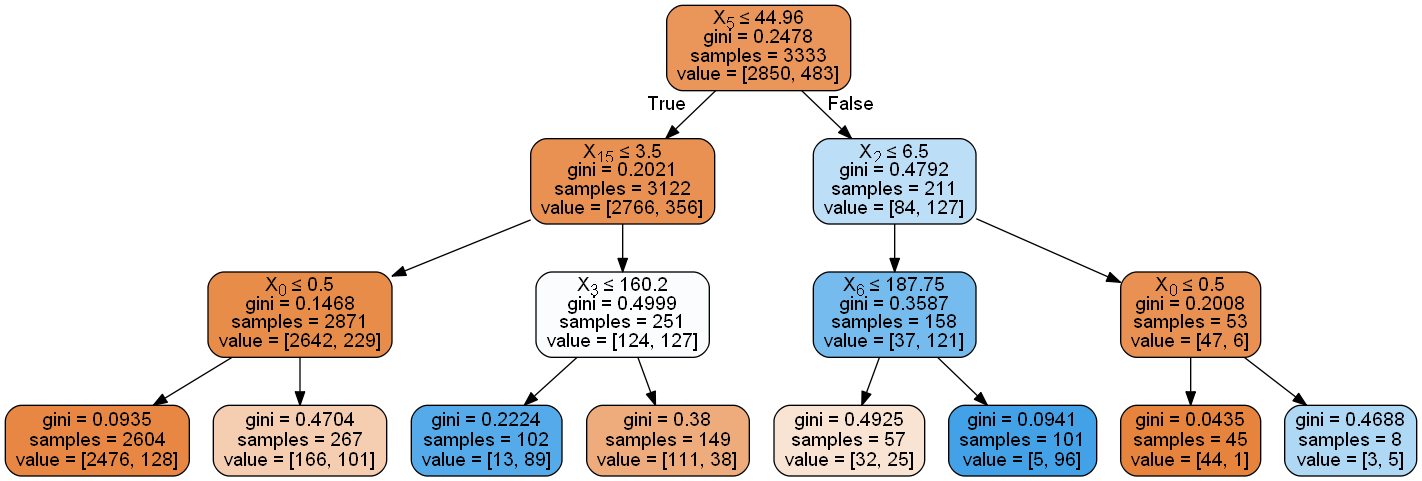
dt = tree.DecisionTreeClassifier(max_depth=3 )
dt.fit(X, y)
print (numpy.sum(y== dt.predict(X)) / len(y))
dot_data = tree.export_graphviz(dt, out_file=None ,
filled=True , rounded=True ,
special_characters=True )
graph = pydotplus.graph_from_dot_data(dot_data)
Image(graph.create_png())
正確率的計算方法有二accuracy_score(iris.target, predicted)numpy.sum(y== dt.predict(X)) / len(y)
混洧矩陣 from sklearn.metrics import confusion_matrixconfusion_matrix(iris.target, predicted)
不同的正確率計算方式from sklearn.metrics import classification_reportprint(classification_report(iris.target, predicted))
precision
recall
f1-score
support
0
1.00
1.00
1.00
50
1
0.98
0.90
0.94
50
2
0.91
0.98
0.94
50
avg / total
0.96
0.96
0.96
150